
A Brief Introduction to Natural Language Processing by Ahmet Arda Karabacak
The contemporary generative AI tools, either used with directly given prompts or indirectly via AI-integrated applications, change daily life and learning habits.
“In the past decade, natural language processing has become embedded in our daily lives: automatic machine translation is ubiquitous on the web and in social media; text classification keeps our email inboxes from collapsing under a deluge of spam; search engines have moved beyond string matching and network analysis to a high degree of linguistics sophistication; dialog systems provide an increasingly common and effective way to get and share information.” (Eisenstein, 2019, p.1)
When we think and try to find solutions to how such mechanisms can work, one of the first questions we come across is how these tools understand reality. How do they understand what is told to them? What mechanisms make them capable of understanding abstract, complex meanings? The answer to these questions can be drawn from the field of natural language processing (NLP).
With its simplest description, NLP is the endeavour of computational modelling of human language. It is a subfield of artificial intelligence and is the bridge between language and technology. Research has been made to systemize and create a set of rules for NLP through different machine learning (ML) approaches. The main goal is to get machines to “understand” natural language. With this process, the manipulation of natural language input is achieved (Chowdhary, 2020; Eisenstein, 2019).
I will explain what NLP researchers’ main focus points are:
1. Speech recognition
2. Speech synthesis
3. Natural language understanding
4. Natural language generation
Before beginning, it is essential to learn the history of NLP because each approach adds to the previous one, and it will be easier to concretize more abstract mechanisms, which I will introduce in the future.
1. History of natural language analysis and processing
The analysis of spoken language and beyond, which is understanding it in a given context, has been a point of research for a long time. The journey of linguistic data analysis applications began with machine translation in the first half of the 20th century (Jones, 1994).
1.1 Rule-based approach
One of the first influential experiments in machine translation history is the Georgetown-IBM experiment in 1954. The result of the experiment demonstrated fully automatic translation of 60+ Russian sentences into English. This major success drew great attention and encouraged governments to invest in the field of machine translation and computational linguistics. The newly invented computers were referred to as ‘giant brains’, ‘bilingual machine’.
After the great success, it was expected that within a few years, translating all languages and ‘solving’ this machine translation problem would be possible (Hutchins, 2006).
The method used is called rule-based NLP. Rule-based machine translations (RBMT) are the earliest systems. They follow a knowledge-based approach. That is, linguistic experts manually build translation lexicons using dictionaries and grammar books. They consist of strict rules of complex syntax and grammar created by professionals.
1.2 Machine Learning & Statistical models
Up until the 1980s, NLP systems were rule-based. In the 1980s, the emergence of ML algorithms for language processing revolutionized NLP. These algorithms, with increasing computational power (see Moore’s law), allowed faster and larger data processing. With the processing of large bilingual text corpora, statistical models emerged. The infrastructure of statistical machine translation (SMT) is built on information theory. A translation is made according to the probability that a word ‘x’ in the target language is the translation of the word ‘y’ in the source language.
I will not go into the details of the probabilistic distribution of these translation models. Rather, I will give an example to make things more concrete:
The main method is to analyze the co-occurrence frequency. That is, the frequency with which certain patterns occur together. To calculate this, conditional probability is used.
⭕ Conditional probability is the probability of ‘b’ following if ‘a’ occurs, with ‘a’ being a word in the source language, and ‘b’ a word in the target language = P(b|a)à[0,1]
To simplify this: P(b|a) = #(b, a)/#(a), i.e., number of times ‘b’ and ‘a’ occur together, out of all times ‘a’ occurs (Brown et al., 1993).
Let us exemplify this with a small pattern recognition exercise:
jī tāng = chicken soup
lǎo yā táng = duck soup
suān là tāng = hot and sour soup
In this example, when we calculate P(soup|tāng) with the formula given above, we have the outcome 3/3. This means that ‘soup’ is an equivalent of ‘tāng.’
| 1. Number of times ‘tāng’ occurs | #(tāng) = 3 |
| 2. Number of ‘soup’ occurs together with ‘tāng’ | #(soup, tāng) = 3 |
| 3. Probability of ‘tāng’ and ‘soup’ occur together. i.e., P(soup|tāng) | P(soup|tāng) = #(soup, tāng)/#(tāng) = 3/3 = 100% |
In simple words, statistical models learn through statistical probability by being trained on lots and lots of data
!Do not forget that this is an overly simplified example, and that statistical models have many more components other than co-occurance freq, such as word alignment (Brown et al., 1993) and n-grams (Jurafsky, D., Martin, J.H., 2026).
1.3 Neural Networks
Neural networks (NNs) are far more complex and abstract compared to the previous models. I would like to note that understanding the mechanism of NNs is very important for understanding modern NLP research, especially in the generative AI field. This is because neural networks are fundamental for two critical aspects of how LLMs work. The first is word embeddings, which is how LLMs ‘understand’ the meaning of lexical items and their relationship with each other in a given context. The second is Transformers, which are also neural network models that solve the problem of pronoun resolution, long-distance dependencies, discourse structure, large context windows, and many more.
I will explain what word embeddings and Transformers are in a different text, in which I will talk about how LLMs ‘understand’ and generate natural language. For now, I will introduce the basic concepts of NNs very briefly, and not get into the technical or mathematical details.
Neural networks can be compared to a computer model of the human brain and nervous system (although this is a disputed analogy). The study has been inspired by the complex webs of interconnected neurons of natural learning systems. How NN architectures work is similar to human neurons work. The output of artificial neurons mimic biological ones: the output is dependent on the stimuli they receive from other neurons and the strength of the connection. This means that the input of a neuron can be an output of another neuron (Mitchell, T. M., 1997).
Think of the neuron as a placeholder for a number. A word cannot be placed in a neuron. It has to be a numerical representation. This number may represent a color, a word, or something else. I will give an example to make this more concrete:
A simple task that uses NN is image recognition. What is done in image recognition is converting the image to a sequence of numbers. This is done by giving each pixel a number depending on its color. This sequence of numerical representations is fed into the network. The outcome is a prediction (Jurafsky, D., Martin, J.H., 2026).
Now that you know the fact that neurons hold numbers, I will explain the architecture of a small neural network.
There are layers called the hidden layers in between the input layer and the prediction. Each connection between the input layer and the neuron in the hidden layer also has a specific learned weight. Weight is, in simple words, a multiplier used while calculating the number outcome of the neuron in the hidden layer. The outcome of the calculation is a single number.
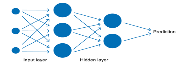
For example, an image of a dog is fed into the network. The system could predict if it’s a cat or a dog.
The question “how does the system identify the dog?” may arise now. The answer is that the network is trained on a huge amount of data. This is a good example of ‘supervised learning’: The system has a cyclical process through which it improves its prediction with each false label it gives. By doing this repeatedly, the system learns that some features are more important than others to give good predictions.
There is one important note: the feature weights may not be explicitly modeled; the system may learn them by itself. This is one of the major reasons why LLMs have gender biases.
Because a deeper explanation would require mathematics and make the text wander off the subject, this much information about neural networks is more than enough.
2. NLP Applications
Rightfully, until now, the topic may be confused with machine translation. However, it’s beneficial to know that NLP research began with machine translation and then turned into the well-known LLM fields with the approach of Transformer structures. That is why I did not start with explaining how language generation originated. Furthermore, ML models are simply tools that help identify patterns and make predictions, and form the foundational basis of MT.
Even though it may be hard to understand the mechanics of daily used NLP applications without knowing their infrastructure materials, it is possible to know the applications themselves and where they are used by basically looking around the world we live in.
2.1. Automatic Speech Recognition
Also called speech-to-text, this application is useful when generating automatic captions for audio/video.
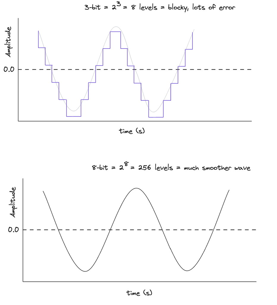
Think of the waveforms as a set of trees or mountains. A machine cannot ‘see’ a waveform. It has to idealize and numerize it. Thus, to create audio signals, the computer puts dots on the fractions of speech data to generate a waveform (Jurafsky, D., Martin, J.H., 2026). Each of these dots is a discrete number that represents the amplitude of a specific spot in the wave. The machine analyzes those dots to create a spectrogram. Check the image below:
The generated spectrogram is fed into a neural network called an acoustic model, which is specifically trained on audio. The acoustic model calculates and predicts the most probable phoneme according to the vectors it has been fed. I would like to clarify that the algorithm is only predicting phonemes for now due to connected speech. Before going to the next stage, the combined phonemes are separated using a massive pronunciation lexicon (gathered from phonetically annotated corpora or pronunciation dictionaries).
The predictions with the highest probability score are sent to a language model, which is a neural network trained on text corpora. The language model, at this stage, is merely a henchman that predicts (I will talk more about this in detail in my next articles) and ‘checks’ whether the correlations are related when the orthography is transcribed (Yu, D., Deng, L., 2016).
To understand better and continue further, I would like to introduce the terms AM score and LM score. The AM score is a numerical score of the most probable phoneme sequence. LM score is a numerical score of the most probable keyword in context. AM score is more important than LM score because it provides the phonemes and their sequence, and as I said before, the LM is merely a henchman. That is, the LM score comes into play when the AM is ‘confused’ by background noise, homophone words, etc.
The last check is a hypothesis search which combines AM and LM scores and outputs the word sequence with the highest score (Yu, D., Deng, L., 2016).
Let me give a simple example of the process:
Let’s take the utterance ‘I am a child’ into consideration. First, this utterance is recorded and fed into the audio tokenizer. The machine generates the spectrogram according to its acoustic features (Hz, amplitude, etc.). The spectrogram is fed into the acoustic model, and the most probable phonemes are the output:
/aɪæmətʃaɪld/ (diphthongs are generated as singular phonemes because of the constant glide of the pitch. They are not generated as combinations of different, singular vowel sequences.)
The sequence of phonemes is decoded with algorithms, and the most probable combinations that match the lexicon are found. Every combination probability is calculated and assigned an AM score. Then, they are sent to the LM.
LM, in this example, is useful for differentiating the homophones ‘eye’ and ‘I’. ‘I’ is chosen because the probability of the sentence starting with ‘I’ is higher. I will explain the details of this in my next article about the mechanisms of language generation. The next words are generated mainly according to the AM score.
2.2. Text-to-speech
Text-to-speech (also called TTS or speech synthesis) is used in a variety of fields, such as language model interaction, speech production, and reading text out loud for those with neurological disorders. One famous example of this may be Stephen Hawking, who depended on TTS technology after losing use of his voice.
In the past, hundreds of hours of speech data were collected from a single talker. Thus, the resulting system only worked in one voice. For a second voice, data must have been collected from a second talker. Today, to create speech with an unseen voice, very small amounts of speech from the desired talker are used to guide the voice creation.
The mechanism is a reversal of ASR: When a sentence is fed into the algorithm, the orthography is transcribed into a sequence of phonemes using a lexicon.
The input text is a sequence of characters. This text is broken into separate sentences by a sentence-splitting algorithm, and the sentence boundaries are found. Each sentence is then further divided into a sequence of tokens. The words found are taken and are encoded as phonemes (Taylor, P., 2009).
This whole process, of course, requires training. The TTS systems use language models for text tokens and an audio tokenizer based on an audio codec to tokenize a vast amount of speech data.
⭕ A codec is a coder/decoder. An audio codec is the standard way of learning audio tokens. It encodes analog speech signals into a digitized compressed representation that can be stored and sent. For TTS, they are used for converting speech into tokens (Jurafsky, D., Martin, J.H., 2026).
Then, the model is trained to take two input sequences, a text transcript and a sample of speech, tokenize both into discrete tokens, and generate samples of speech corresponding to the text string. Lastly, with a decoder, these tokens are converted into a waveform.
TTS systems and the outputs are evaluated by humans. The utterance is played to listeners, and they are asked to give a mean opinion score (MOS), basically a rating of how good the utterance was. Then, the systems are compared with their sentences’ MOS. If there are exactly two systems to be compared, a comparative MOS (CMOS) method could be used. That is, listeners give scores according to which of the two utterances is better.
2.3. Natural Language Understanding
Language understanding begins with preprocessing, a process of preparing a text for specific computational analysis. Some preprocessing steps are:
- Sentence splitting: Sentence boundaries are identified in the text using cues like capital letters, punctuation, etc. Rule-based approaches are used.
- Tokenization: Text is broken into smaller units like words, subwords, or characters. Tokenization tools are already implemented in existing software packages such as spaCY. I will talk about the details of text tokenization approaches in my next article.
Once preprocessing is done, morphological analysis begins. This is for understanding the structure and formation of words by analyzing affixes and root words. Morphological analysis is mandatory because word construction implies word meaning. - Part-of-Speech (PoS) tagging is used to assign grammatical categories to each word. When encountering an unfamiliar word, morphological clues are crucial. It is important to note that this is a hybrid method that is also a syntactic analysis because of the English grammar.
Example: “The garage was crammed with old bicycles.”→ determiner, noun, verb, verb, preposition, adjective, noun, punctuation mark
⭕ Do not forget that these analyses do not refer to words. They refer to tokens. That is why the full stop is also analysed.
After morphological analysis, syntactic analysis begins. The grammatical structure of a sentence is analyzed to determine the relationships between words and their roles within the sentence.
- Chunking (shallow parsing): Meaningful phrases are extracted from the phrase by grouping words into syntactically related units like noun phrases (NP), verb phrases (VP), etc., using PoS tagging. Chunking is a form of constituency parsing.
⭕ Syntactic analysis has two types:
1. Constituency parsing, which is based on phrase structure rules (PSR) of the language. A sentence is analyzed via the hierarchical tree structure of constituents. Constituents are groups of words that behave as single units made by the chunking methodology.
2. Dependency parsing, which is based on the grammatical relationships between words. Relations may be described with respect to a predicate, e.g., “I” is nsubj (check Universal Dependency Relations) with respect to the verb “prefer”. Or with the ways in which words can modify their heads. E.g., “the” modifies the subj “plane” as a det.
Semantic ambiguity and lexical meaning have been (and still are) a major trouble in the development of natural language understanding in many ways. Most of these problems were solved first with static word embeddings, then contextual word embeddings, and then with Transformer architectures. Semantic analysis allowed:
Semantic role labeling: Identifying and classifying the roles of different lexical items in a sentence with respect to a predicate: “The cat chased the mouse”cat is the agent, while the mouse is the patient.
Word sense disambiguation: Determining the correct meaning of a word with multiple possible interpretations in a specific context.
Named entity recognition: Identifying and classifying named entities (real-world objects like locations, people, etc.) in context. One good example could be the name: George Bush. It could be a person, or a bush named George.
Discourse analysis has been the most problematic one. Indeed, LLMs still do not have the capabilities of humans in terms of understanding. The Transformers architecture improved language understanding from a small window to a large window, with which now LLMs can understand and remember hundreds of pages at the same time. One of the major problems solved by discourse analysis is:
– Coreference resolution: Identifying and linking mentions in a text that refer to the same entity: “Sara was talking to her supervisor about her new project.” In this example, the pronoun ‘her’ refers to Sara. Even for humans, it is not easy to understand this, and it may cause discussions.
These were the crucial steps in NLP to grasp the meaning of words and improve text understanding. In my next article, I will not go over these steps, nor explain them again. I will continue by giving more details about them and linking those details to LLMs.
2.4. Natural Language Generation
Before jumping into the topic of Natural Language Generation, I’d like to confess that I find this introductory text rather long. Thus, I plan to make my next article solely about language generation. The details of the topics mentioned in this article will be in the next article, along with the process of language generation.
References and Further Readings
- Brown, P., Cocke, J., Pietra, S. D., Pietra, V. D., Jelinek, F., Mercer, R., & Roossin, P. (1988). A statistical approach to language translation. Proceedings of the 12th Conference on Computational Linguistics -. https://doi.org/10.3115/991635.991651
- Brown, P.F., Pietra, S.D., Pietra, V.J., & Mercer, R.L. (1993). The Mathematics of Statistical Machine Translation: Parameter Estimation. Comput. Linguistics, 19, 263-311.
- Chowdhary, K.R. (2020). Natural Language Processing. In: Fundamentals of Artificial Intelligence. Springer, New Delhi. https://doi.org/10.1007/978-81-322-3972-7_19
- Daniel Jurafsky and James H. Martin. 2026. Speech and Language Processing: An Introduction to Natural Language Processing, Computational Linguistics, and Speech Recognition with Language Models, 3rd edition. Online manuscript released January 6, 2026. https://web.stanford.edu/~jurafsky/slp3.
- Eisenstein, J. (2019). Introduction to natural language processing. The MIT Press.
- Hutchins, J. (2006). The first public demonstration of machine translation: the Georgetown-IBM system, 7th January 1954.
- Information is based on the “Translation Technology” and “NLP and Linguistic Analysis” classes given by Prof. Dr. Lieve Macken and Janiça Hackenbuchner in UGent
- Jones, K. S. (1994). Natural language processing: a historical review. Current issues in computational linguistics: in honour of Don Walker, 3-16.
- Mitchell, T. M. (1997). Machine learning. Mcgraw-Hill. https://www.cs.cmu.edu/~tom/files/MachineLearningTomMitchell.pdf
- Taylor, P. (2009). Text-to-Speech Synthesis. Cambridge: Cambridge University Press.
- Yu, D., & Deng, L. (2016). Automatic speech recognition (Vol. 1). Berlin: Springer.


Leave a Reply